 Fraxlend
 interest rates respond to utilization through each pair's configured calculator
Fraxlend interest rates determine borrowing costs separately for each isolated pair through its configured rate calculator. Utilization drives the calculation, while variable models also account for elapsed time and rate history. The quoted rate can therefore change while a loan remains open and interest adds to its debt.
Updated -
Read the quote for the selected pair
A borrowing quote belongs to a particular asset-collateral pair and the calculator that prices its loans. Start with the selected pair's lending asset, collateral token, and rate model. Another pair can quote a different rate even when it lends the same asset, because its utilization and calculator settings differ. A figure shown beside a lending position describes a different relationship: the return on supplied assets.
Keep the rate's time unit attached when comparing quotes. An annualized percentage expresses the current borrowing pace over a year; it does not fix that pace for the loan's duration. Comparing figures from different moments can also hide a utilization change between those observations.
Utilization and the available asset balance
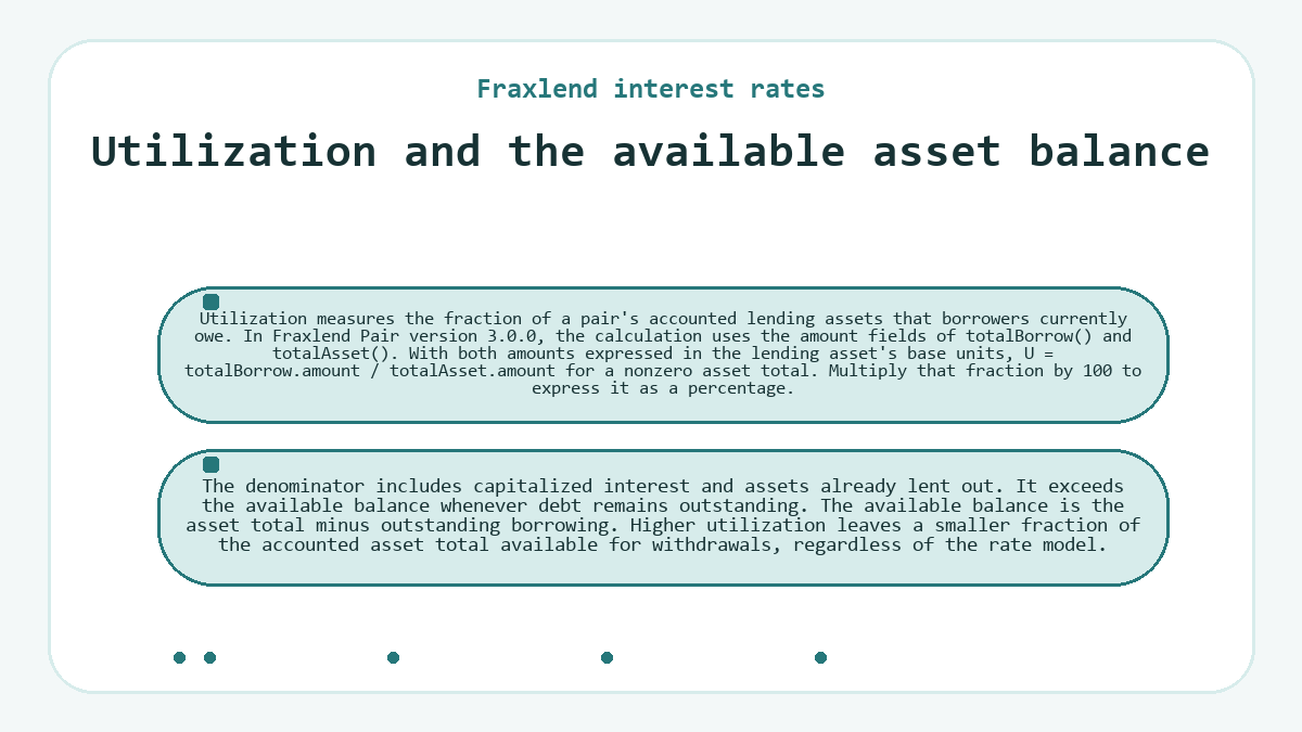
Utilization measures the fraction of a pair's accounted lending assets that borrowers currently owe. In Fraxlend Pair version 3.0.0, the calculation uses the amount fields of
totalBorrow()
and
totalAsset()
. With both amounts expressed in the lending asset's base units,
U = totalBorrow.amount / totalAsset.amount
for a nonzero asset total. Multiply that fraction by
100
to express it as a percentage. The denominator includes capitalized interest and assets already lent out. It exceeds the available balance whenever debt remains outstanding.
The available balance is the asset total minus outstanding borrowing. Higher utilization leaves a smaller fraction of the accounted asset total available for withdrawals, regardless of the rate model.
The Linear Rate's fixed curve
The Linear Rate maps utilization onto two connected straight segments, with the vertex marking where the slope changes. Its settings specify the rate at zero utilization, the vertex rate, the vertex utilization, and the rate at full utilization. Below the vertex, the curve connects the minimum and vertex rates. Above it, the curve connects the vertex and maximum rates.
For these formulas,
U
and
U_vertex
express utilization as fractions, and all rates use the same time unit.
Below vertex utilization, the Linear Rate calculates
r = r_min + U * (r_vertex - r_min) / U_vertex
.
At the vertex itself, the rate equals
r_vertex
. Above it,
r = r_vertex + (U - U_vertex) * (r_max - r_vertex) / (1 - U_vertex)
. The Linear Rate fixes these curve settings at creation, so repeating a utilization reading on that unchanged curve gives the same rate.
The time-weighted rate's target range
The Time-Weighted Variable Rate changes its borrowing rate over time according to a target utilization range. Utilization below that range pushes the rate downward; utilization above it pushes the rate upward. Within the target range, this model leaves the rate unchanged. Minimum and maximum rate settings bound the adjustment, while the configured half-life governs its speed.
A half-life describes rate adjustment under its specified utilization condition. For this model, it measures the time required for the rate to halve at zero utilization, subject to the minimum rate. It does not describe the time for a borrower's debt to double. Away from zero utilization, the actual response depends on the utilization reading.
Variable Rate V2 and its changing curve
Variable Rate V2 combines an immediate utilization response with a curve that adjusts over elapsed time. Movement along the curve changes the borrowing quote as utilization changes. Sustained utilization outside the target range changes the full-utilization rate, which also changes the vertex rate. Future quotes therefore depend on the curve's stored state.
The target range controls curve adjustment; the vertex marks the join between the curve's linear segments.
Within the target range, the full-utilization rate stays unchanged, although movement along the existing curve still changes the borrowing rate. Below the range, the full-utilization rate decreases; above it, that rate increases. Configured bounds constrain the full-utilization rate. The half-life controls adjustment speed, while the distance from the target range also affects the response.
When zero utilization falls below the target range, one update spanning the half-life halves the full-utilization rate, subject to its minimum. When full utilization exceeds the target range, one update spanning the half-life doubles the full-utilization rate unless its maximum bound limits the increase. These endpoint rules concern the curve parameter; the rate at another utilization also reflects its location on the curve.
Position changes and their rate effects
Debt repayment reduces the balance exposed to future interest, while adding collateral improves loan-to-value without reducing that balance. These Fraxlend Pair version 3.0.0 comparisons hold other balances constant and exclude interest accrued during the transaction.
| Position or market action | Effect on utilization and access |
|---|---|
| Supply more Asset Tokens | Adds to the asset total and lowers utilization when debt is outstanding; the pair must permit the deposit. |
| Redeem fTokens | Reduces the asset total and raises utilization when debt remains; redemption requires available liquidity and an unpaused withdrawal function. |
| Borrow additional Asset Tokens | Raises utilization; the borrower needs permitted borrowing capacity and sufficient available assets. |
| Repay Asset Tokens | Reduces outstanding borrowing and utilization; repayment reduces the selected borrower's debt and requires an unpaused repayment function. |
| Add Collateral Tokens | Changes collateral backing without directly changing utilization; the borrowed balance remains exposed to interest when accrual is active. |
Repayment can lower future interest charges by shrinking the debt even before the market quote moves. Additional collateral addresses the liquidation threshold through LTV. Neither action gives one borrower control over other participants' borrowing or the calculator's future output.
Accrued interest and the repayment balance
Capitalized interest increases the debt represented by a borrower's existing shares, so repayment includes interest as well as principal. In Fraxlend Pair version 3.0.0, an active accrual update calculates pair-wide interest from elapsed seconds, outstanding borrowing, and the calculator's returned rate. With
r
expressed as an unscaled per-second fraction, the relationship is
I = B * r * t
. Here,
B
is pair-wide debt before the update, and
t
is elapsed seconds. An interest pause prevents this calculation while active.
When interest capitalizes, both asset and borrow amounts grow while borrow shares remain unchanged. With unchanged collateral value, a growing debt raises loan-to-value (LTV) and brings the loan closer to its liquidation threshold.
Why does the lending return differ from the borrow rate?
The lending return spreads borrower interest across all supplied asset claims, including the portion that remains available in the pair.
Only borrowed assets generate borrower interest, so a lender's return also reflects utilization. Where a protocol interest fee applies, it further reduces the interest attributable to existing lenders. Fraxlend Pair version 3.0.0 accounts for this fee as a fraction of accrued borrower interest and issues corresponding asset shares. Its calculation base is interest, not the whole deposit. The interest allocation appears in the underlying value represented by fTokens. Comparing a borrow quote directly with a supply return therefore mixes different denominators.
Rate exposure over the borrowing period
Rate predictability depends on both the calculator's rules and how long borrowing remains outstanding. A fixed Linear Rate curve makes the response to a given utilization reading reproducible. The variable models add adjustment over time, so recent rate history can explain a current quote without establishing the next quote. Continued borrowing, repayments, new lending, and withdrawals can change the inputs during the holding period.
A rate cap bounds the calculator's output within its applicable configuration; it does not independently cap a loan's total interest. Keeping debt open still incurs costs based on its balance, applicable rates, and duration. Decide whether the selected pair's rate behavior fits the intended borrowing period, including possible utilization or curve changes before repayment.
Fraxlend interest rates - common questions
Does zero utilization mean the borrowing calculator returns a zero rate?
Zero utilization does not require a zero borrowing rate. Variable Rate V2 has a configured ZERO_UTIL_RATE, while the Linear Rate uses its configured minimum at zero utilization. If there is no outstanding borrowing, there is no borrower debt generating interest for lenders.
Can a pair's configured rate calculator change after deployment?
Fraxlend Pair version 3.0.0 permits the timelock authority to replace the rate calculator unless that setter has been revoked. The pair exposes isRateContractSetterRevoked to identify that restriction. An ordinary borrower does not control this setting, and a calculator's own fixed parameters do not establish that the pair must always use it.
Does a lower borrowing rate undo interest that has already accrued?
A lower borrowing rate does not reverse interest that has already capitalized into the debt. It changes the rate used for applicable subsequent accrual calculations. Repayment still covers the outstanding amount, including earlier interest, so a falling quote and a debt balance above the original principal can occur together.
Are collateral prices direct inputs to the interest-rate calculators?
Fraxlend's calculators price interest from utilization, with variable models also using elapsed time or prior rate state. Collateral prices enter the separate loan-health calculation through the oracle exchange rate. They can affect borrowing behavior and therefore utilization indirectly, but a collateral price move alone does not specify a new borrowing rate.
Do I need a transaction just to preview accrued interest?
A read-only call to previewAddInterest() can show projected interest without changing Fraxlend Pair version 3.0.0 state. It also returns projected rate information and asset and borrow accounting. The preview does not save those values; a state-changing accrual call updates the stored accounting when the contract permits interest accrual.